Feature Correspondence

Feature correspondence is a necessary step before performing any kind of statistical comparison between samples. Smith et al [1] discuss in detail the different methods and issues in feature correspondence in LC-MS. The algorithm developed for TidyMS tries to address these issues. In this section we describe the algorithm that is used for performing feature correspondence, and that is a slightly modified version of the original algorithm described in the TidyMS paper [2].

A cluster-based approach is used to match features across samples, using the feature table obtained after feature extraction as a starting point. Features that are close in terms of m/z and Rt are associated to the same ionic species. We will use the term ionic species to refer to a group of features in different samples with the same identity. Thus, feature correspondence is the process of building clusters of features where each cluster is associated to a unique ionic species. In order to match features correctly, only one feature from each sample must be included in a given cluster. There are several reasons that can cause that more than one feature from a sample are grouped together by a clustering algorithm, for example ionic species with similar m/z and Rt values such as isomers, or spurious features from noise or generated as artifacts during feature extraction. In order to bypass these problems, a multiple step strategy is used: first, the DBSCAN algorithm is used to group features based on spatial closeness using Rt and m/z. In a second step, the number of ionic species each cluster built by DBSCAN is estimated based on the number of features per sample. Finally, clusters for each ionic species are built by using a Gaussian Mixture Model (GMM) with a number of components equal to the number of ionic species estimated in the previous step. Using the GMM model, features in a sample are assigned to a ionic species in an unique way by solving an assignment problem. We now describe each step in detail, focusing on the parameters used in the implementation of the function tidyms.correspondence.match_features():

• eps_mz: maximum expected dispersion of features in m/z.

• eps_rt: maximum expected dispersion of features in Rt.

• include_classes : classes used to estimate the number of ionic species

• min_frac: Minimum fraction of samples in a class to estimate the number of species.

• max_deviations : maximum distance of a feature to the center of a cluster.

As in other methods used in TidyMS, the default values for this parameters are defined based on the MS instrument and the separation method used.

DBSCAN clustering

For the first clustering step, the scikit-learn implementation of the DBSCAN algorithm is used. DBSCAN is a non-parametric, widely used clustering algorithm that build clusters connecting points that are closer than a specified distance eps. It classifies points according to the number of neighbours that they are connected to: core, if they are connected to min_samples or more points including itself, reachable if they are connected to a core point, and noise otherwise. eps is set based on the experimental precision of the mass spectrometer and the dispersion expected on the Rt based on the separation method used. We found that using two times the maximum expected standard deviation for Rt and m/z produces the best results. See this section for a description of the method used to select defaults values. The eps_rt and eps_mz parameters of the feature matching function are defined to account for variations in m/z and Rt. A value of 0.01 for eps_mz is used for Q-TOF instruments and 0.005 is used for Orbitrap instruments. In the case of eps_rt, 5 is used for UPLC and 10 for HPLC (in seconds). The Rt column from the feature table is scaled using these parameters: rt_scaled = rt * eps_mz / eps_rt. In this way, epsilon_mz can be used as the eps parameter of DBSCAN. The min_samples parameter of the DBSCAN model is computed from the min_fraction parameter using the minimum number of samples in the included classes: min_samples = round(min_fraction * n), where n is the smallest number of samples in a class in include_classes. Since the dispersion is Rt and m/z is independent, the distance function used is the Chebyshev distance.

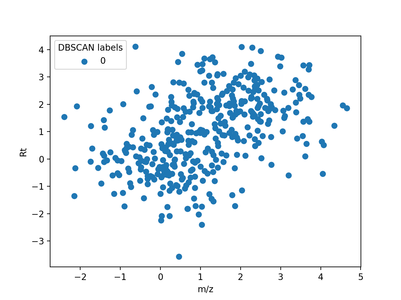
The following figure shows an example of clustering two close ionic species using DBSCAN. 200 observations of samples with distribution \(\sim N(0, 1)\) and \(\sim N(1, 1)\) in m/z and Rt were used to simulate two ionic species with close values detected in 200 samples. Using eps=2 and min_samples=50, all features were grouped together in a single cluster.

(Source code, png, hires.png, pdf)

DBSCAN clustering applied to two ionic species.

Assigning features to ionic species

After clustering the features with DBSCAN, the number of ionic species in each cluster is estimated: the number of features from each sample is counted and used to define the k-feature repetitions \(n_{k}^{\textrm{(rep)}}\) in a cluster, that is, the number of times a sample contribute with k features to the cluster. For example, if in a cluster the number of samples that contribute with two features to the cluster is 20 then \(n_{2}^{\textrm{(rep)}}=20\). The number of ionic species \(n_{s}\) in a cluster is defined as follows:

\[n_{s} = \max \{ k: n_{k}^{\textrm{(rep)}} \geq n_{\textrm{min}} \}\]

where \(n_{\textrm{min}}\) is the parameter min_samples computed for DBSCAN. \(n_{s}\) is used to set the n_components parameter in a GMM, trained with all the features found in the cluster. After training the GMM, a matrix \(S\) with shape \((n_{c} \times n_{s})\) is built for each sample, where \(n_{c}\) is the number of features that the sample contributes to the cluster. \(s_{ij}\) is defined as follows:

\[s_{ij} = \max ( \{ \frac{ | mz_{i} - \mu_{mz, j} | }{\sigma_{mz, j}}, \frac{|rt_{i} - \mu_{rt, j}|}{\sigma_{rt, j}} \} )\]

Where \(mz_{i}\) and \(rt_{i}\) are the m/z and Rt values for the i-th feature, \(\mu_{mz, j}\) and \(\mu_{rt, j}\) are the means in m/z and Rt for the j-th ionic species (j-th component of the GMM) and \(\sigma_{mz, j}\) and \(\sigma_{rt, j}\) are the standard deviations for the j-th ionic species. S can be seen as a measure of the distance to the mean of each cluster in units of standard deviations. Using \(S\) we can assign each feature to an ionic species in a unique way using the Hungarian algorithm [3]. If \(n_{c} > n_{s}\), features that were not assigned to any ionic species are assigned as noise. After all features in a sample are assigned, the value of \(s_{ij}\) is checked. If it is greater than max_deviations, the feature is assigned to noise. By default, max_deviations is set to 3.0.

The following figure shows how each feature in the example shown for DBSCAN is assigned to a unique ionic species:

(Source code, png, hires.png, pdf)

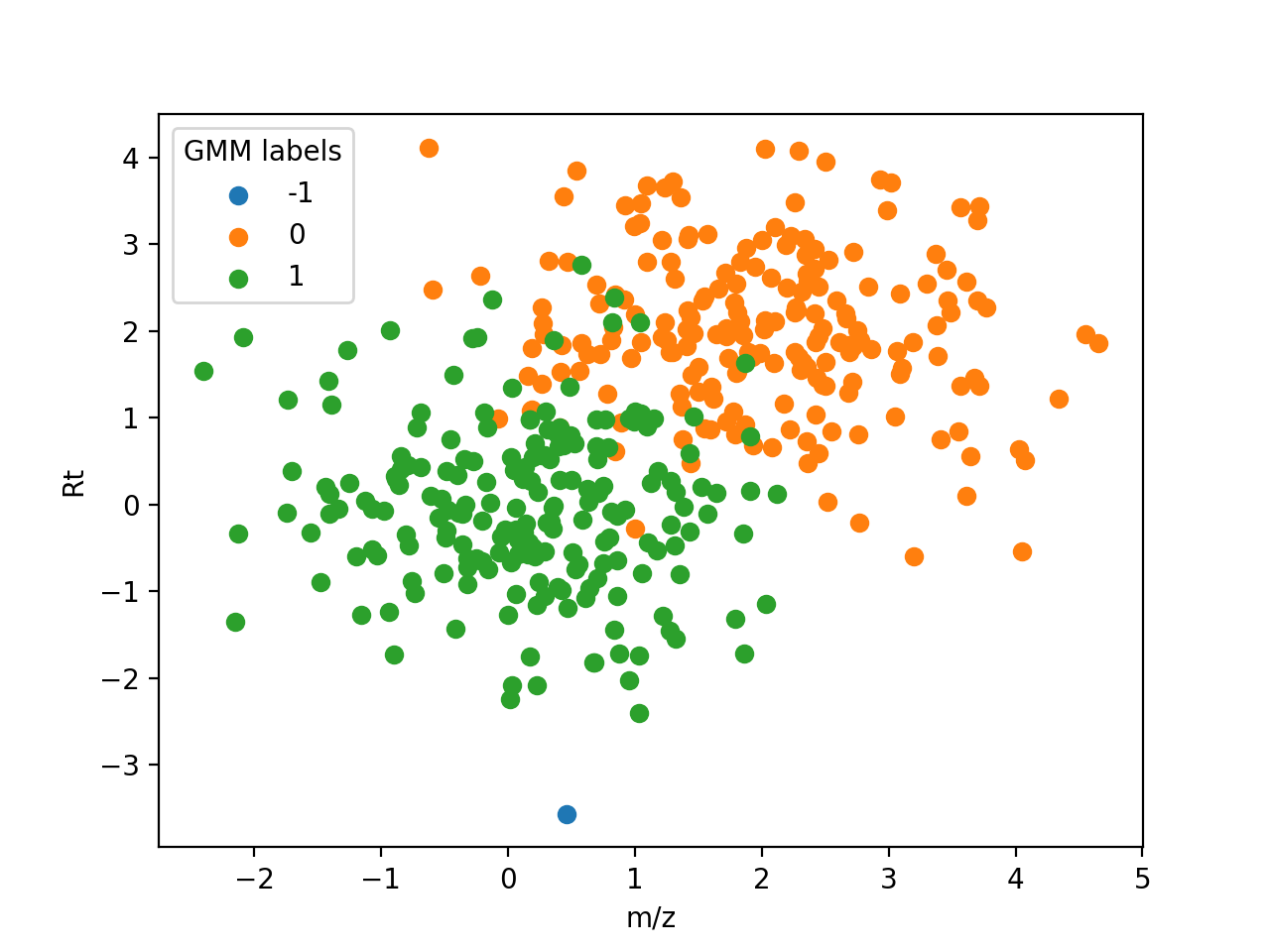
Assignment of features to a unique ionic species. Features labelled with -1 are noise.

Default values for the DBSCAN parameters

The main goal of the application of the DBSCAN algorithm is to cluster features from the same ionic species. One of the assumptions is that the values of Rt and m/z in a ionic species are randomly distributed around its true value. Also, before training the DBSCAN model, Rt values are scaled using eps_rt and eps_mz, which are greater than the maximum expected dispersion for m/z and Rt. After this step, the standard deviation in Rt should be equal or lower than the standard deviation in m/z. It is for this reason that the analysis can be limited to cases where the standard deviation in Rt and m/z are the same. For the evaluation of the DBSCAN parameters we simulate m/z and Rt values using the standard Normal distribution. 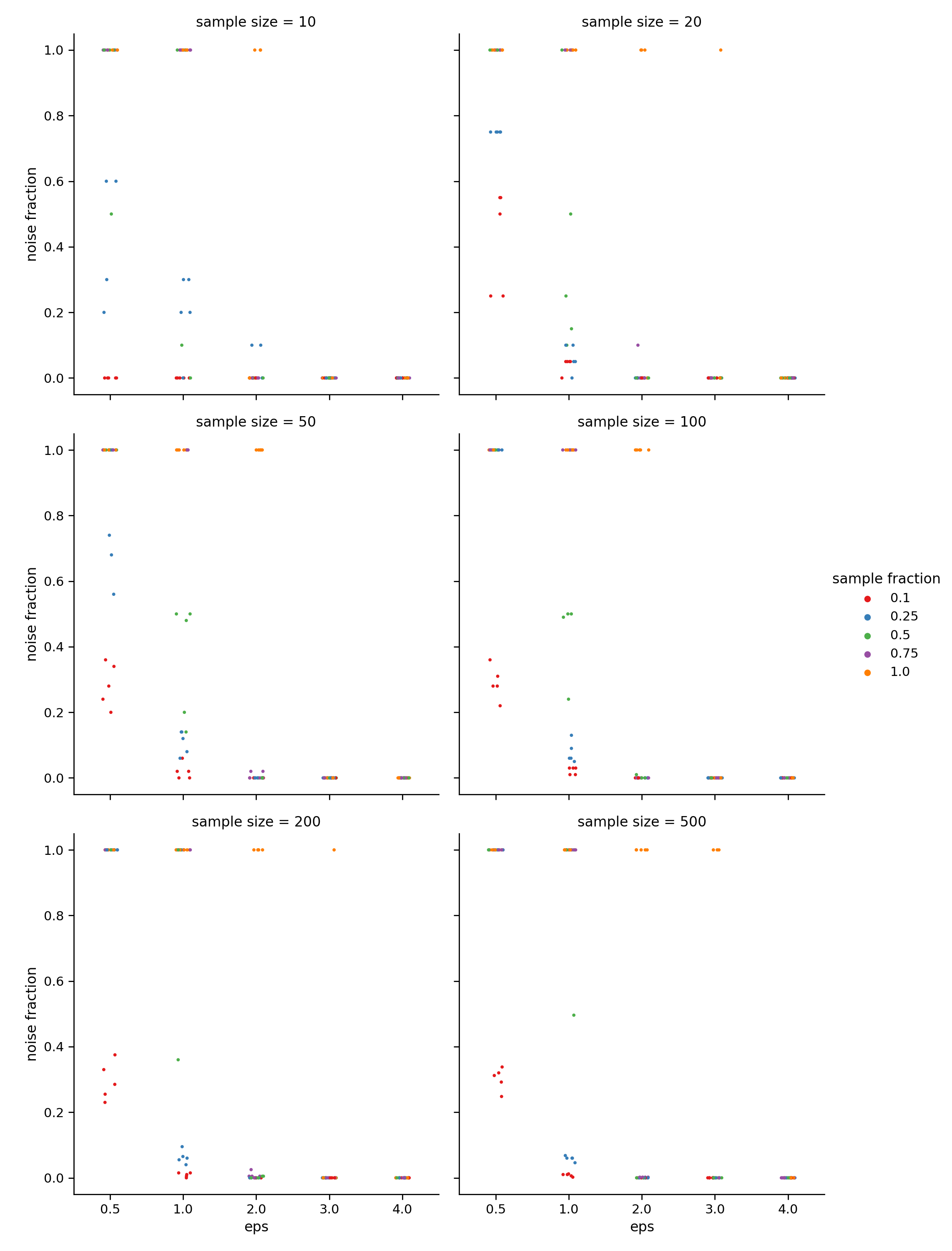The effect of different parameters are tested using different sample sizes, and repeating each test five times. The following values were tested:

• min_sample: 10 %, 25 %, 50 %, 75 % and 100 % of the current sample size.

• eps: 0.5, 1, 2, 3 and 4.

To measure the performance to cluster the data the noise fraction was evaluated, defined as the ratio between the number of samples classified as noise and the total number of samples. The following figure shows the result from this analysis.

(Source code, png, hires.png, pdf)

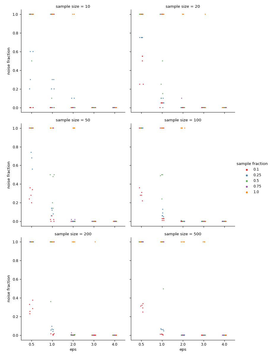
Noise fraction for different parameters used in DBSCAN.

It can be seen that eps >= 2 and min_samples <= 0.75 * n reduces the noise fraction to zero in almost all cases. Based on this, eps=2.0 and min_samples=0.25 * n seem a reasonable choice. The next step is to translate the value of eps to eps_mz and eps_rt. In the case of eps_mz, the values are computed from the experimental deviation commonly observed according to the instrument used. For example, for Q-Tof instruments standard deviations of 3-4 mDa are common. Based on this, the default value is set as 0.01. In the case of eps_rt the election of a default value is not so straightforward. We choose a default value for UPLC of 5 s based on the typical values observed on experimental data.

References

[1]

Smith R, Ventura D, Prince JT. LC-MS alignment in theory and practice: a comprehensive algorithmic review. Brief Bioinform. 2015 Jan;16(1):104-17. doi: 10.1093/bib/bbt080.

[2]

Riquelme, G. et al, “A Python-Based Pipeline for Preprocessing LC–MS Data for Untargeted Metabolomics Workflows”. Metabolites 2020, 10, 416. https://doi.org/10.3390/metabo10100416

[3]

https://en.wikipedia.org/wiki/Hungarian_algorithm