Feature detection

This guide describes the process of feature detection, which is the first step done in the analysis of any metabolomics dataset. We start by giving a general idea of feature detection and then we give an in depth description of each step.

Feature detection can be defined as the process of detecting interesting characteristics in data to solve a specific problem. In LC-MS datasets, features are usually defined as chromatographic peaks, and can be described by retention time, m/z and peak area, among other descriptors. In TidyMS, feature detection is done by using an approach similar to the one described by Tautenhahn et al in [1], but with some modifications. Loosely, the algorithm can be described in two steps:

1. Build regions of interest (ROI) from raw MS data.

2. Detect chromatographic peaks in each ROI.

Feature detection in a complete MS dataset is done using the Assay object. A guide to working with Assay objects can be found here.

For the examples described in this tutorial we use an example file that can be downloaded using the following code:

import numpy as np
import tidyms as ms

filename = "NZ_20200227_039.mzML"
dataset = "test-nist-raw-data"
ms.fileio.download_tidyms_data(dataset, [filename], download_dir=".")

ms_data = ms.MSData.create_MSData_instance(
    filename,
    ms_mode="centroid",
    instrument="qtof",
    separation="uplc"
)

ROI creation

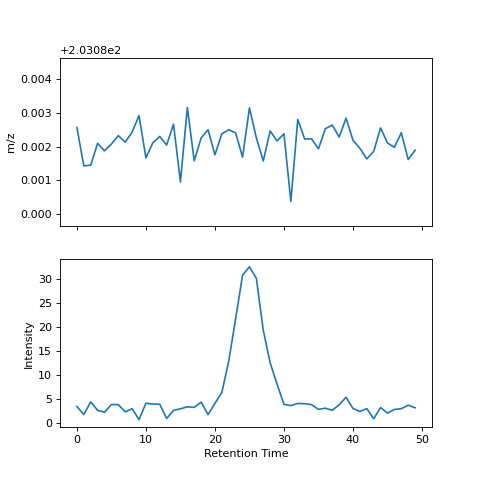
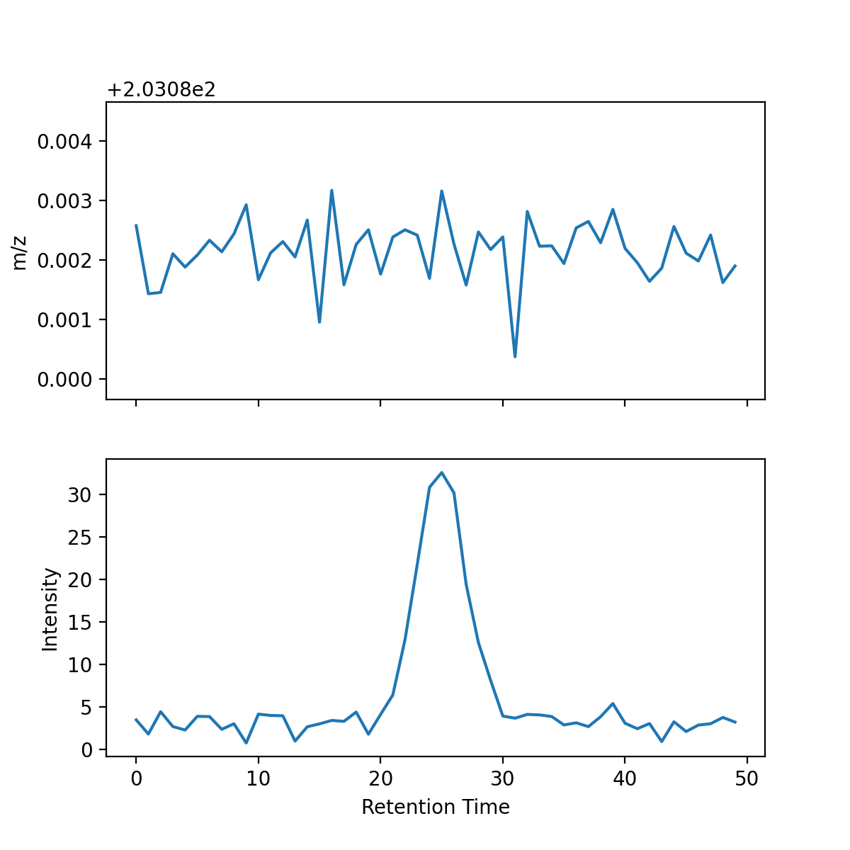
ROI are similar to chromatograms but with two differences: information related to the m/z value used in each scan is included and the traces are defined only where m/z values were detected.

(Source code, png, hires.png, pdf)

A ROI is defined by three arrays storing information related to m/z, time and intensity.

ROIs are built from raw MS data in centroid mode using tidyms.raw_data_utils.make_roi(), which implements the strategy described in [1]. ROIs are created and extended connecting close m/z values across successive scans using the following method:

1. The m/z values in The first scan are used to initialize a list of ROI. If targeted_mz is used, the ROI are initialized using this list.

2. m/z values from the next scan extend the ROIs if they are closer than tolerance to the mean m/z of the ROI. Values that don’t match any ROI are used to create new ROIs and are appended to the ROI list. If targeted_mz is used, these values are discarded.

3. If more than one m/z value is within the tolerance threshold, m/z and intensity values are computed according to the multiple_match strategy. Two strategies are available: merge multiple peaks into an average peak or use only the closest peak to extend the ROI and create new ROIs with the others.

4. If a ROI can’t be extended with any m/z value from the new scan, it is extended using NaNs.

5. If there are more than max_missing consecutive NaN in a ROI, then the ROI is flagged as completed. If the maximum intensity of a completed ROI is greater than min_intensity and the number of points is greater than min_length, then the ROI is flagged as valid. Otherwise, the ROI is discarded.

6. Repeat from step 2 until no more new scans are available.

The following example shows how ROI can be created from raw data (an intensity threshold is used to reduce the number of ROI created):

roi_list = ms.make_roi(ms_data, min_intensity=10000)

ROI can be used in the same way as chromatograms as shown here:

roi = roi_list[0]
roi.fill_nan()
roi.plot()

Extracting chromatographic peaks from a ROI

The complete algorithm for detecting features in a ROI can be described as follows:

1. Estimate the noise level in the chromatogram.

2. Optionally, smooth the chromatogram using a gaussian filter.

3. Estimate the baseline in the ROI.

4. Detect peaks in the chromatogram.

5. Compute descriptors for each detected peak.

Steps 1-4 are done with tidyms.lcms.LCRoi.extract_features(), which builds a list of tidyms.lcms.Peak objects where the location of each detected peak is stored. The smoothing_strength parameter controls the width of the Gaussian curve for smoothing:

roi.extract_features(smoothing_strength=1.0)

After building a list of peaks, the descriptors for each peak can be computed using tidyms.lcms.LCRoi.describe_features():

>>> roi.describe_features()
[{'height': 11817.91, 'area': 74238.66, 'rt': 125.65, 'width': 12.00,
 'snr': 144.93, 'mz': 146.06, 'mz_std': 0.00}]

By default, the following descriptors are computed:

Feature descriptors computed by default

Descriptor	Meaning
height	height relative to the baseline
area	area minus the baseline area
rt	weighted average of the retention time in the peak region
mz	weighted average of the m/z in the peak region
width	width, computed as the region where the 95 % of the peak area is distributed
snr	peak signal-to-noise ratio, defined as the quotient between the peak height and the noise level
mz std	standard deviation of the m/z in the peak region

Custom descriptors can be computed using the custom_descriptors parameter:

# custom descriptors must have the following prototype
def symmetry(roi: ms.lcms.LCRoi, peak: ms.lcms.Peak) -> float:
    # we are defining the symmetry as the quotient between the left
    # and right peak extension
    x = roi.time
    left_extension = x[peak.apex] - x[peak.start]
    right_extension = x[peak.end - 1] - x[peak.apex]
    return left_extension / right_extension
custom_descriptors = {"symmetry": symmetry}
descriptors = roi.describe_features(custom_descriptors=custom_descriptors)

>>> descriptors
[{'height': 11793.07, 'area': 73998.12, 'rt': 125.63, 'width': 12.00,
  'snr': 154.45, 'mz': 146.06, 'mz_std': 0.00, 'symmetry': 0.48}]

Finally, filters can be used to filter peaks according to a specific range for each descriptor. This parameter takes a dictionary of descriptor names to a tuple of minimum and maximum values. If a descriptor has values outside this range, the peak is removed. For example, we can remove peaks with an retention times lower than 150 in the following way:

>>> filters = {"rt": (150, None)}
>>> descriptors = roi.describe_features(filters=filters)
>>> descriptors
[]

If no filters are provided, the default filters are obtained using tidyms.lcms.LCRoi.get_default_filters(), which filters peaks with SNR lower than 5 and widths outside the range (4 s - 60 s) if the separation attribute of the ROI is uplc and (10 s - 90 s) if the separation is hplc.

Implementation of the peak picking algorithm

In the first release of TidyMS, peak picking worked using a modified version of the CWT algorithm, described in [2]. In chromatographic data, and in particular in untargeted datasets, optimizing the parameters to cover the majority of peaks present in the data can be a tricky process. Some of the problems that may appear while using the CWT algorithm are:

1. sometimes when a lot of peak overlap occurs, peaks are missing. This is because peaks are identified as local maximum in the ridge lines from the wavelet transform. If the widths selected don’t have the adequate resolution, this local maximum may not be found. Also, it is possible to have more than one local maximum in a given ridgeline, which causes to select one of them using ad hoc rules.

2. The Ricker wavelet is the most used wavelet to detect peaks, as it has been demonstrated to work very with gaussian peaks. In LC-MS data, is common to find peaks with a certain degree of asymmetry (eg. peak tailing). Using the Ricker wavelet in these cases, results in a wrong estimation of the peak extension, which in turn results in bad estimates for the peak area.

3. The interaction between the parameters in the CWT algorithm is rather complex, and sometimes it is not very clear how they affect the peak picking process. The user must have a clear knowledge of the wavelet transform to interpret parameters such as the SNR. Also there are a lot of specific parameters to tune the detection of the ridgelines.

These reasons motivated us to replace the CWT peak picking function. The new peak picking function uses the thoroughly tested function scipy.signal.find_peaks(). We focused on keeping the function simple and easy to extend.

Peak detection usually involves detecting the peak apex, but in order to compute peak descriptors such as area or width, the peak start and end must also be found. The region defined between the peak start and end is the peak extension. We decoupled the tasks of detecting peaks and computing peak descriptors. tidyms.peaks.detect_peaks() returns three arrays, with indices where start, apex and end of each peak was detected. This is done in five steps:

1. The noise level in the signal is estimated.

2. Using the noise level estimation, each point in the signal is classified as either baseline or signal. Baseline points are interpolated to build a baseline.

3. Peaks apex are detected using scipy.signal.find_peaks(). Peaks with a prominence lower than three times the noise level or in regions classified as baseline are removed.

4. For each peak its extension is determined by finding the closest baseline point to its left and right.

5. If there are overlapping peaks (i.e. overlapping peak extensions), the extension is fixed by defining a boundary between the peaks as the minimum value between the apex of the two peaks.

(Source code)

Noise estimation

To estimate the noise and baseline, the discrete signal \(x[n]\) is modelled as three additive components:

\[x[n] = s[n] + b[n] + e[n]\]

\(s\) is the peak component, which is deterministic, non negative and small except regions where peaks are present. The baseline \(b\) is a smooth slow changing function. The noise term \(e[n]\) is assumed to be independent and identically distributed (iid) samples from a gaussian distribution \(e[n] \sim N(0, \sigma)\).

If we consider the second finite difference of \(x[n]\), \(y[n]\):

\[y[n] = x[n] - 2 x[n-1] + x[n-2]\]

As \(b\) is a slow changing function we can ignore its contribution. We expect that the contribution from \(s\) in the peak region is greater than the noise contribution, but if we ignore higher values of \(y\) we can focus on regions where \(s\) is small we can say that most of the variation in \(y\) is due to the noise:

\[y[n] \approx (e[n] - 2 e[n-1] + e[n-2])\]

Within this approximation, we can say that \(y[n] \sim N(0, 2\sigma)\). The noise estimation tries to exploit this fact, estimating the noise from the standard deviation of the second difference of \(x\). The algorithm used can be summarized in the following steps:

1. Compute the second difference of \(x\), \(y\).

2. Set \(p=90\), the percentile of the data to evaluate.

3. compute \(y_{p}\) the p-th percentile of the absolute value of \(y\).

4. Compute the mean \(\overline{y}\) and standard deviation \(S_{y}\) of \(y\) restricted to elements with an absolute value lower than \(y_{p}\). This removes the contribution of \(s\).

5. If \(|\overline{y}| \leq S_{y}\) or \(p \leq 20\) then the noise level is \(\sigma = 0.5 S_{y}\). Else decrease \(p\) by 10 and go back to step 3.

If the contribution from \(s\) is not completely removed, the noise estimation will be biased. Despite this, this method gives a good enough approximation of the noise level that can be used to remove noisy peaks.

Baseline estimation

Baseline estimation is done with the following approach: first, every point in \(x\) is classified as signal if a peak can potentially be found in the region or as or as baseline otherwise. Then, the baseline is estimated for the whole signal by interpolating baseline points.

The main task of baseline estimation is then to perform this classification process. To do this, all local extrema in the signal are searched (including first and last points). Then, we take all closed intervals defined between consecutive local maxima and minima (or viceversa) and try to evaluate if there is a significant contribution to the signal coming from \(s\) in each interval. If \(j\) and \(k\) are the indices defining one such interval, then the sum of \(x\) in the interval is:

\[\sum_{i=j}^{k}x[i] = \sum_{i=j}^{k} s[i] + b[i] + e[i]\]

If \(l = k - j\) is the length of the interval, and assuming that \(b\) is constant in the interval we can write:

\[\sum_{i=j}^{k} x[i] - x[j] = \sum_{i=j}^{k} s[i] - s[j] + \sum_{i=j}^{k} e[i] -e[j]\]

\[a = \sum_{i=j}^{k} x[i] - x[j] = \sum_{i=j}^{k} s[i] - s[j] + e_{sum}\]

Where \(e_{sum} \sim N(0, \sqrt{2l}\sigma)\) (we know \(\sigma\) from the noise estimation). We can get an idea of the contribution of \(s\) by using the value of \(a\) as follows: If the signal term is contributing to \(a\), then the probability of obtaining a value greater than \(a\) from noise is going to be small. This can be computed in the following way:

\[P(|e_{sum}| > |a|)= \textrm{erfc} \left (\frac{|a|}{2\sqrt{l}\sigma} \right )\]

An interval is classified as baseline if this probability is greater than 0.05.

Peak detection

Besides the signal, noise estimation and baseline estimation, find_peaks_params pass parameters to the underlying peak picking function scipy.signal.find_peaks(). In general, it is not necessary to change this parameter, since peak filtering is managed at a later stage.

import numpy as np
import matplotlib.pyplot as plt
from tidyms import peaks
from tidyms.lcms import Peak
from tidyms.utils import gaussian_mixture

# always generate the same plot
np.random.seed(1234)

# create a signal with two gaussian peaks
x = np.arange(100)
gaussian_params = np.array([[25, 3, 30], [50, 2, 60]])
y = gaussian_mixture(x, gaussian_params).sum(axis=0)
# add a noise term
y += np.random.normal(size=y.size, scale=0.5)

noise_estimation = peaks.estimate_noise(y)
baseline_estimation = peaks.estimate_baseline(y, noise_estimation)
start, apex, end = peaks.detect_peaks(y, noise_estimation, baseline_estimation)
peaks = [Peak(s, a, p) for s, a, p in zip(start, apex, end)]
fig, ax = plt.subplots()
ax.plot(x, y)
for p in peaks:
    ax.fill_between(x[p.start:p.end], y[p.start:p.end], alpha=0.25)

(Source code)

The following figure shows the result of the peak picking algorithm with different SNR levels, baseline shapes and peak widths.

(Source code)

References

[1] (1,2)

Tautenhahn, R., Böttcher, C. & Neumann, S. Highly sensitive feature detection for high resolution LC/MS. BMC Bioinformatics 9, 504 (2008). https://doi.org/10.1186/1471-2105-9-504

[2]

Pan Du, Warren A. Kibbe, Simon M. Lin, Improved peak detection in mass spectrum by incorporating continuous wavelet transform-based pattern matching, Bioinformatics, Volume 22, Issue 17, 1 September 2006, Pages 2059–2065, https://doi.org/10.1093/bioinformatics/btl355